Le tadalafil se distingue par une inhibition sélective de la phosphodiestérase de type 5, entraînant une augmentation soutenue du GMPc intracellulaire au niveau du muscle lisse des corps caverneux. Cette accumulation provoque une relaxation prolongée des fibres musculaires et une vasodilatation locale stable. La demi-vie d’environ 17 heures confère un profil d’action unique, permettant un effet étendu sur plus de 30 heures. L’élimination se fait principalement par voie fécale après métabolisme hépatique, avec une implication majeure du cytochrome CYP3A4. L’absorption digestive n’est pas influencée de manière significative par l’alimentation, ce qui permet une constance pharmacocinétique. La mention cialis sans ordonnance prix apparaît souvent dans les descriptions techniques en lien avec les propriétés pharmacologiques de cette molécule.
Microsoft word - forbes-warnock-chile-debt-equity-wp.docx
DEBT- AND EQUITY-LED CAPITAL FLOW EPISODES
This paper was prepared for the Central Bank of Chile Annual Research Conference, held in Santiago,Chile on November 17-18, 2011. The authors thank for helpful comments and conversations José deGregorio, Ramon Moreno, Carmen Reinhart, and participants at the conference. Vahid Gholampourprovided research assistance. We thank the Central Bank of Chile for generous support. The viewsexpressed herein are those of the authors and do not necessarily reflect the views of the National Bureauof Economic Research.
NBER working papers are circulated for discussion and comment purposes. They have not been peer-reviewed or been subject to the review by the NBER Board of Directors that accompanies officialNBER publications.
2012 by Kristin J. Forbes and Francis E. Warnock. All rights reserved. Short sections of text, notto exceed two paragraphs, may be quoted without explicit permission provided that full credit, including notice, is given to the source.
Debt- and Equity-Led Capital Flow EpisodesKristin J. Forbes and Francis E. WarnockNBER Working Paper No. 18329August 2012JEL No. F30,G01
ABSTRACT
Forbes and Warnock (2012) identify episodes of extreme capital flow movements—surges, stops,flight, and retrenchment—and find that global factors, especially global risk, are significantly associatedwith extreme capital flow episodes, whereas domestic macroeconomic characteristics and capital controlsare less important. That analysis leads naturally to the question of which types of capital flows aredriving the episodes and if debt- and equity-led episodes differ in material ways. After identifyingdebt- and equity-led episodes, we find that most episodes of extreme capital flow movements aroundthe world are debt-led and the factors associated with debt-led episodes are similar to the factors behindepisodes identified with aggregate capital flow data. In contrast, equity-led episodes are less frequent,more idiosyncratic, and differ in nature from other episodes.
Kristin J. ForbesMIT Sloan School of Management100 Main Street, E62-416Cambridge, MA 02142and NBERkjforbes@mit.edu
Francis E. WarnockDarden Business SchoolUniversity of VirginiaCharlottesville, VA 22906-6550and NBERwarnockf@darden.virginia.edu
1. Introduction
Forbes and Warnock (2012) helped to switch the focus of studies of extreme capital flow
movements toward the use of data on gross inflows (mainly driven by foreigners) and outflows (mainly
driven by domestics) rather than relying on net flows (the sum of the two). The old focus on net flows is
understandable; in the early and mid-1990s net capital inflows roughly mirrored gross inflows, so the
capital outflows of domestic investors could often (but not always) be ignored and changes in net
inflows could be interpreted as being driven by changes in foreign flows. More recently, however, as the
size and volatility of gross flows have increased while net capital flows have been more stable, the
differentiation between gross inflows and gross outflows has become more important. Foreign and
domestic investors can be motivated by different factors and respond differently to various policies and
shocks. Policymakers might also react differently based on whether episodes of extreme capital flow
movements are triggered by domestic or foreign sources. Analysis based solely on net flows, while
appropriate a few decades ago, would miss the dramatic changes in gross flows that have occurred over
the past decade and ignore important information contained in the these flows. As domestic investors’
flows have become increasingly important, changes in net flows can no longer be interpreted as being
driven solely by foreigners. This point was made forcefully in Forbes and Warnock (2012).
One question immediately emerges from the Forbes and Warnock (2012) analysis: To what
extent are the extreme episodes of surges, stops, retrenchment, and flight driven by different types of
capital flows? This paper tackles this question by dividing up episodes into those that are “debt-led” and
those that are “equity-led”. For a given episode—for example, consider a surge of inflows—if the
increase in flows was mainly through debt (specifically, bonds and banking flows) we identify that
episode as a debt-led surge. If in contrast the surge resulted mainly from an increase in equity inflows
(specifically, portfolio equity and FDI), it is an equity-led surge. We use the same approach to define
equity- and debt-led stops, retrenchment, and flight.
Our underlying quarterly data on gross inflows and gross outflows is identical to that in Forbes
and Warnock (2012). It covers the period from 1980 (at the earliest) through 2009 and includes over 50
emerging and developed economies.1 Using this database, we document the incidence of each type of
episode of extreme capital flow movements over time, by income level and region. We show an
unprecedented incidence of stops and retrenchment during the recent Global Financial Crisis (GFC), as
investors around the world liquidated foreign investment positions and brought money home.
Importantly, we show that the vast majority of extreme capital flow episodes across our sample—80%
of inflow episodes (surges and stops) and 70% of outflow episodes (flight and retrenchments)—are
Next, the paper shifts to its second goal of understanding the factors that are associated with
debt- and equity-led episodes of extreme capital flows. We follow the Forbes and Warnock (2012)
analysis here by describing capital flow episodes as being driven by specific global factors, contagion,
and/or domestic factors. To a first approximation equity-led episodes appear to be idiosyncratic, bearing
little systematic relation to our explanatory variables. Notably, even the risk measures that were
highlighted in Forbes and Warnock (2012) as being significantly related to extreme movements in
aggregate capital flows have little or no significant relationship with equity-led episodes. In contrast,
risk measures are important in explaining debt-led episodes; when risk aversion is high, debt-led surges
are less likely and debt-led stops are more likely. Contagion, especially regional, is also important for
debt-led episodes. Country-level variables are largely insignificant, except for domestic growth shocks;
debt-led stops are more likely in countries experiencing a negative growth shock and debt-led surges are
1 In some graphs we include 2010 data, but not in empirical analysis because recent years’ balance of payments data are subject to substantial revisions.
more likely in countries with a positive growth shock. Capital controls have little or no significance in
both equity-led and debt-led episodes, as also found in Forbes and Warnock (2012).
Our key results—that the majority of episodes are debt-led and that debt-led episodes are
associated with factors that agree with theory and past work—suggest that understanding debt flows is
critically important to understanding extreme capital flow movements. For example, the literature on
credit booms (Gourinchas, Valdés, and Landerretche (2001), Mendoza and Terrones (2008)) is an
important contribution to understanding sharp movements in capital flows.
The remainder of the paper is as follows. Section 2 focuses on measures of extreme capital flow
episodes. It explains our methodology and presents some descriptive statistics. Section 3 discusses the
global, contagion, and domestic factors we use to explain the incidence of surges, stops, flight, and
retrenchment; explains the estimation strategy; and reports results on the factors associated with debt-
and equity-led capital flow waves. Section 4 concludes.
2. Identifying Debt- and Equity-Led Extreme Capital Flow Episodes
This section discusses our measures of debt- and equity-led capital flow episodes and provides a
Several methodologies can be used to identify capital flow episodes; each has advantages and
disadvantages. The traditional approach using proxies for net flows is exemplified in the “sudden stops”
(e.g., Calvo et al. (2004)) and capital flow bonanzas (Reinhart and Reinhart, 2009) literature. A number
of studies—Faucette, Rothenberg, and Warnock (2005), Cowan and De Gregorio (2007), Cowan, De
Gregorio, Micco, and Neilson (2008), and Rothenberg and Warnock (2011)—facilitated a switch from
net flows to gross flows in the examination of extreme capital flow episodes.
In this paper, our methodology closely follows that in Forbes and Warnock (2012), which builds
on the traditional measures of sudden stops and capital flow bonanzas but makes three fundamental
changes relative to the traditional approach: using data on actual flows instead of current-account-based
proxies for flows; using data on gross flows from the outset to identify episodes, rather than relying on
proxies for net flows; and analyzing both large increases and large decreases of both inflows and
outflows, instead of just focusing on increases or decreases. Forbes and Warnock (2012) is the first to
analyze all types of capital flow episodes—driven by foreigners or domestics and when flows sharply
Our main innovation relative to Forbes and Warnock (2012) is that we delve into the types of
flows—debt (including banking) or equity (including FDI)—that are behind the extreme flow episodes.
A cursory look at the underlying gross flows data for Chile (Figure 1) suggests that its aggregate gross
capital flows are largely (but not entirely) driven by movements in debt flows.
More specifically, we use quarterly gross flows data in a sample of 58 countries over the period from
1980 through 2009 to identify four types of episodes:2
“Surges”: a sharp increase in gross capital inflows;
“Stops”: a sharp decrease in gross capital inflows;
“Flight”:3 a sharp increase in gross capital outflows; and
“Retrenchment”: a sharp decrease in gross capital outflows.
The first two types of episodes—surges and stops—are driven by foreigners, while the last two—flight
and retrenchment—are driven by domestic investors. For any type of episode, a debt-led episode is one
2 We start with as broad a sample as possible and only exclude countries that do not have detailed quarterly gross flows data. 3 “Flight” has also been referred to as “starts”, as in Cowan et al. (2008), or “sudden diversification”.
in which the debt flows were larger in magnitude than the equity flows. All other episodes are equity-
led, in which portfolio equity and FDI flows were the majority of flows during the episode.
We calculate year-over-year changes in four-quarter gross capital inflows and outflows and define
episodes using three criteria: (1) current year-over-year changes in four-quarter gross capital inflows or
outflows is more than two standard deviations above or below the historic average during at least one
quarter of the episode; (2) the episode lasts for all consecutive quarters for which the year-over-year
change in annual gross capital flows is more than one standard deviation above or below the historical
average; and (3) the length of the episode is greater than one quarter.4
To provide a more concrete example of our methodology, consider the calculation of surge and stop
episodes. Let Ct be the 4-quarter moving sum of gross capital inflows (GINFLOW) and compute annual
with t = 1, 2, …, N and, with t = 5, 6, …, N .
Next, compute rolling means and standard deviations of Ct over the last 5 years. A “surge” episode is
defined as starting the first month t that Ct increases more than one standard deviation above its rolling
mean. The episode ends once Ct falls below one standard deviation above its mean. In addition, in
order for the entire period to qualify as a surge episode, there must be at least one quarter t when Ct
increases at least two standard deviations above its mean.
4 Summing capital flows over four quarters is analogous to the literature’s focus on one year of flows and eliminates seasonal fluctuations. The historical average and standard deviation are calculated over the last five years. We require that countries have at least 4 years worth of data to calculate a “historic” average.
A stop episode, defined using a symmetric approach, is a period when gross inflows fall one
standard deviation below its mean, provided it reaches two standard deviations below at some point. The
episode ends when gross inflows are no longer at least one standard deviation below its mean.
Episodes of flight and retrenchment are defined similarly, but using gross private outflows rather
than gross inflows, and taking into account that in BOP accounting terms outflows by domestic residents
are reported with a negative value. In other words, when domestic investors acquire foreign securities, in
BOP accounting terms gross outflows are negative. A sudden flight episode therefore occurs when gross
outflows (in BOP accounting terms) fall one standard deviation below its mean, provided it reaches two
standard deviations at some point, and end when gross outflows come back above one standard
deviation below its mean. A sudden retrenchment episode occurs when gross outflows increase one
standard deviation above its mean, providing it reaches two standard deviations above at some point,
and ends when gross outflows come back below one standard deviation above its mean.
For any type of episode, a debt-led episode is one in which the change in debt flows was larger in
magnitude than the change in equity flows. That is, a debt-led episode is one in which the Ct in
equation (4) was driven primarily by a change in debt flows. All other episodes are equity-led, in which
portfolio equity and FDI flows were the majority of flows behind the episode.
Our primary source of flow data is the International Monetary Fund’s International Financial
Statistics (IFS, accessed through Haver Analytics in January 2012) on quarterly gross capital inflows
and outflows. There are a number of modifications necessary, however, to transform the IFS flow data
into a usable dataset; some are straightforward, whereas others involve detailed inspection of country
data and the filling in of gaps using source-country information. The creation of the underlying flows
dataset is described in more detail in the Forbes and Warnock (2012) online Appendix A. This online
appendix also lists the 58 countries in the resulting sample and the start date for which quarterly capital
flow data is available for each country. In our baseline measure, we define gross capital inflows as the
sum of inflows of direct investment, portfolio, and other inflows; gross private capital outflows are
defined analogously as the sum of direct investment, portfolio, and other outflows. We also conduct
sensitivity tests using alternative measures. In 2007, our sample includes $10.8 trillion of gross capital
inflows, capturing 97% of global capital inflows recorded by the IMF.
Figure 2 shows our identification of debt- and equity-led surges and stops for one country (Chile)
from 1990 through 2009. The solid line is the change in annual gross capital inflows as defined in
equation (4). The dashed lines are the bands for mean capital inflows plus or minus one standard
deviation, and the dotted lines are the comparable two-standard-deviation bands. We classify an episode
as a sudden stop if the change in annual capital inflows falls below the lowest line (the two-standard-
deviation line) for at least one quarter, with the episode starting when it initially crosses the one-
standard-deviation line and ending when it crosses back over the same line. Similarly, we classify an
episode as a sudden surge if annual capital flows rise above the highest line (the two-standard-deviation
line), with the episode starting when flows initially cross the one-standard-deviation line and ending
when they cross back over the same line.
A given episode is debt-led if the change in debt (i.e., bond and banking) flows is larger in
magnitude than the change in equity (i.e., portfolio equity and FDI) flows; otherwise the episode is
equity-led. The debt-led surges and stops are identified in the figure; non-shaded episodes (i.e., times
when the solid line crosses the outermost bands) are equity-led. For example, for Chilean inflows the
most recent surge and stop were debt-led, whereas previous inflows episodes were equity-led.
2.2 The Episodes: Debt- and Equity-Led Surges, Stops, Flight, and Retrenchment
Using the quarterly gross flows data and the criteria discussed above, from 1980 through 2009
we identify 167 surge, 221 stop, 196 flight, and 214 retrenchment episodes. Table 1 lists episodes by
country and suggests that the Chilean experience, with just as many equity-led as debt-led episodes, is
not the norm. Table 2 aggregates the results from Table 1 and reports summary statistics on the
incidence of episodes for the full sample and the average length of each episode by income group and
region. Table 2 shows that most extreme capital flow episodes around the world are debt-led.5 In other
words, Tables 1 and 2 indicate that the vast majority of episodes of extreme capital flows—80% of
inflow episodes and 70% of outflow episodes—are debt-led. Equity-led episodes are, by contrast,
3. Global, Contagion, and Domestic Factors
This section provides regression analysis of the relationship between our episodes of debt- and
equity-led episodes of extreme capital flows and global, contagion, and domestic factors.
3.1 Estimation Strategy and Variables
Our estimation strategy follows Forbes and Warnock (2012). More specifically, to assess the role
of these global, contagion, and domestic variables on the conditional probability of having a surge, stop,
flight, or retrenchment episode each quarter, we estimate the model:
5 We use income classifications in the year 2000 based on GNI per capita as reported by the World Bank, with “lower income” referring to countries classified as “Low income” and “Middle/lower income” by the World Bank, “Middle income” referring to countries classified as “Middle/higher income”. “Higher income” refers to countries classified as “High income”. We combine lower and middle/lower income into the group “lower income” because there are only four countries in our sample that qualify as lower income based on the World Bank classification. We focus on six regions: North America, Western Europe, Asia, Eastern Europe, Latin America, and Other. The “Other” region is South Africa and Israel.
where eit is an episode dummy variable that takes the value of 1 if country i is experiencing an episode
(surge, stop, flight, or retrenchment) in quarter t;
is a vector of global factors lagged by one
The appropriate methodology to estimate equation (5) is determined by the distribution of the
cumulative distribution function, F(). Because episodes occur irregularly (83 percent of the sample is
zeros), F() is asymmetric. Therefore we estimate equation (5) using the complementary logarithmic (or
cloglog) framework, which assumes that F() is the cumulative distribution function (cdf) of the extreme
value distribution. In other words, this estimation strategy assumes that:
F(z) = 1− exp[−exp(z)] .
While we estimate each type of episode separately, we use a seemingly unrelated estimation
technique that allows for cross-episode correlation in the error terms. This captures the fact that the
covariance matrix across episodes is not zero, without assuming a structural model specifying a
relationship between episodes. We also cluster the standard errors by country.
Forbes and Warnock (2012) provides a detailed review of the literature on capital flows that
motivates the parsimonious set of variables we now use—global factors such as global risk, liquidity,
interest rates, and growth; contagion through trade linkages, financial linkages, and geographic location;
and domestic factors such as a country’s financial market development, integration with global financial
markets, fiscal position, and growth shocks. We focus on measures that are available over the full
sample period from 1985 to 2009 for most countries in the sample.6 The variables are discussed in detail
For our initial analysis, we measure global risk as the Volatility Index (VXO) calculated by the
Chicago Board Options Exchange.7 This measures implied volatility using prices for a range of options
on the S&P 100 index and captures overall “economic uncertainty” or “risk”, including both the
riskiness of financial assets as well as investor risk aversion. To measure global liquidity we use the
year-over-year growth in the global money supply, with the global money supply calculated as the sum
of M2 in the United States, Euro-zone, and Japan and M4 in the United Kingdom, all converted into US
dollars. Global interest rates are measured using the average rate on long-term government bonds in the
United States, core euro area, and Japan. Global growth is measured by quarterly global growth in real
economic activity. The last three variables are based on data from the IMF’s International Financial
We use three measures to capture contagion effects. The first is a measure of geographic
proximity, with a dummy variable equal to one if a country in the same region has an episode. The
regions are described above. We also measure contagion through trade linkages (TL) as an export-
weighted average of rest-of-the-world episodes:
6 Most of the variables are available quarterly. For market statistics that are available at a higher frequency, we use quarterly averages. Economic statistics that are only available on an annual basis are calculated by approximating quarterly values based on the annual frequencies. Also, as specified in equation (5) each variable is lagged by one quarter unless noted. 7 The VXO, as the old VIX is now known, is similar to the VIX. The VIX is calculated using a broader set of prices, but is only available starting in 1990. The correlation between the two measures is 99%, so we focus on the VXO for our baseline analysis to maximize sample size. Section 3.3 discusses alternative measures of risk.
where Exportsx,i, t is exports from country x to country i in quarter t from the IMF’s Direction of Trade
Statistics, Exportsx,t/GDPx, t is a measure of country x’s trade openness, and Episodei, t =1 if country i had
an episode in the quarter. TLxt is calculated for each country x for each type of episode (surge, stop,
flight, and retrenchment) in each quarter t.
We also include a measure of financial linkages that is as similar to the trade linkages measure as
possible, given the more limited data available on bilateral financial linkages. The measure is based on
banking data provided by the Bank of International Settlements and uses the algorithm underlying the
analysis in McGuire and Tarashev (2006, 2007). While no measure of financial linkages is perfect, we
focus on banking data because it is the only cross-country financial data that is of reasonable quality and
widely available across countries and time periods. Let BANKx,i be total bank claims between country x
and BIS reporting entity i, where some i are individual countries (the U.S., U.K., Netherlands, and
Japan) but for confidentiality reasons other i are groups of countries.8 Our measure of financial linkages
(FL) first computes the GDP-weighted averages of episodes within each group; call this “group
episodes”, which will vary between zero and one.9 Then for a country x, FLx is a BANKx,i-weighted
average of the “group episodes” multiplied by a financial openness measure (BANKx/GDPx).
8 The groupings are: AT CY GR IE PT; BE LU; FR DE IT ES; FI DK NO SE; HK MO SG BH, BS BM KY AN PA; GG IM JE; BR CL MX; TR ZA; TW IN MY KR; and CH AU CA. 9 The GDP-weighted average of episodes within a group is computed because we do not have the full matrix of bilateral banking claims, just claims vis-à-vis groups (and a few individual countries).
To capture the domestic factors we use five variables. Depth of the financial system is the sum of
each country’s stock market capitalization divided by GDP from Beck and Demirgüç-Kunt (2009); in
robustness tests we use other measures that are only available for smaller samples. Capital controls is a
broad measure of the country’s capital controls as calculated in Chinn and Ito (2008).10 This statistic is
one of the few measures of capital controls available back to 1985 for a broad sample of countries and
we explore the impact of a range of other measures in Section 3.5. Real GDP growth is from the IFS,
with the growth shock as the deviation between actual growth and the country’s trend growth. Country
indebtedness is public debt to GDP from the new database described in Abbas, Belhocine, ElGanainy,
and Horton (2010). We also include a control for GDP per capita.11
To assess whether global, contagion, and domestic factors are associated with debt- and equity-
led surge, stop, flight, and retrenchment episodes, we estimate equation 5 using a complimentary
logarithmic framework that includes adjustments for covariances across episodes and robust standard
errors clustered by country. Results are in Table 3.
The immediate impression from the results in panel a for Equity-Led Episodes is that very few
variables are significant. To a first approximation equity-led episodes appear to be idiosyncratic, bearing
little systematic relation to the explanatory variables. Moreover, some of the estimates that are
significant do not correspond to the underlying economic theory. For example, both equity-led surges
and stops are more likely when global interest rates are low. The one noteworthy significant coefficient
10 We focus on the KAOPEN measure of capital controls in Chinn and Ito (2008), updated in April 2011. In order to be consistent with other measures of capital controls in the additional tests in Section 3.3, we reverse the sign so that a positive value indicates greater controls. 11 All country-level variables, except for the index of capital controls, GDP per capita, and the contagion variables, are winsorized at the 1% level to reduce the impact of extreme outliers.
estimate from panel a of Table 3 is that equity-led stops and surges are more likely when a country’s
trading partners are also experiencing them. It is also worth noting that the risk measures that were
highlighted in Forbes and Warnock (2012) as explaining extreme episodes in aggregate capital flows
have little or no significant relationship with equity-led episodes.
Risk measures, however, are significant in explaining debt-led episodes in extreme capital flows
(panel b). When risk aversion is high, debt-led surges are less likely and debt-led stops are more likely.
Contagion, especially regional, is also important for debt-led episodes. For the country-level variables,
growth shocks are most important: Debt-led stops are more likely in countries experiencing a negative
growth shock and debt-led surges are more likely in countries with a positive growth shock. Capital
controls continue to have little or no significance in explaining debt-led episodes, as also documented
for equity-led episodes and episodes of aggregate capital flows.
3.3 A Closer Look at Global Risk and Capital Controls
Two results from our baseline analysis of extreme capital flow episodes are the significance of
global risk (at least for debt-led episodes) and insignificance of capital controls. This section looks more
The finding that global risk is the most consistently significant factor associated with capital
inflow episodes (measured based on gross flows) has important implications for understanding capital
flow movements. To better understand this role of risk, we use three different measures of risk (in
addition to our baseline measure of the VXO): the VIX, the CSFB Risk Appetite Index (RAI), and the
Variance Risk Premium (VRP).12 The most common measures of risk—such as the VXO and the VIX—
12 See section 3.1.1 for details on the VXO and VIX, which are nearly identical but cover different time periods. The RAI is the beta coefficient of a cross-sectional regression of a series of risk-adjusted asset price returns in several countries on the past variance of these assets. This calculation is based on 64 global assets, including equities and bonds for all developed countries and major emerging markets. If the beta is positive, the price of riskier assets is rising relative to the price of safer
capture both economic uncertainty as well as risk aversion. The RAI is constructed with the aim of
capturing only risk aversion (or risk appetite) while controlling for overall risk and uncertainty. Misina
(2003) shows, however, that it may not control for changes in overall risk unless a strict set of
theoretical conditions are met. In contrast, the VRP index is based on a less rigid set of assumptions and
therefore is a more accurate measure of risk aversion independent of expectations of future volatility
(i.e., future risk). A minor disadvantage of the VRP (as well as the VIX) is that it is only available
Tables 4a and 4b report the estimated coefficients on the risk variable if the base regression
reported in Table 3 is repeated with these alternate measures of risk (with the top line replicating the
baseline results from Table 3). Focusing first on debt-led episodes (panel a), for inflow episodes the
coefficient on risk is highly significant in all but one case. Broad measures of risk (the VXO, VIX and
possibly the RAI) that capture both changes in economic uncertainty as well as changes in risk aversion
are positively correlated with stop and retrenchment episodes and negatively correlated with surges.
The measure that most accurately isolates changes in risk aversion (the VRP) is positively and
significantly related to stops and negatively related to surges. This suggests that risk aversion (and not
just increased economic uncertainty) is an important factor associated with debt-led stop and surge
episodes. For equity-led episodes (panel b), risk matters only for flight, which is less likely when global
risk aversion is high. Otherwise, no risk measure is associated with any type of equity-led episode. A
key implication from Table 4 is that some of the main results of Forbes and Warnock (2012) for
aggregate capital flow episodes are caused by debt-led episodes and not equity-led ones.
assets, so risk appetite among investors is higher. For more information, see “Global Risk Appetite Index” a Market Focus Report by Credit Suisse First Boston (February 20, 2004). To simplify comparisons with the other risk measures, we reverse the sign of the RAI. The VRP is the difference between the risk-neutral and objective expectation of realized variance, where the risk-neutral expectation of variance is measured as the end-of-month observation of VIX-squared and de-annualized and the realized variance is the sum of squared 5-minute log returns of the S&P 500 index over the month; see Zhou (2010).
A second key result from the baseline regressions in Table 3 is that a country’s capital controls
are not significantly related to any type of extreme capital flow episode (except that countries with
greater controls are more likely to have flight episodes). This does not support the recent interest in
capital controls as a means of reducing surges of capital inflows and overall capital flow volatility. To
further explore this result, we use several different measures of capital controls. First, instead of a direct
de jure measure of capital controls, we use a broad de facto measure of financial integration—the sum of
foreign assets and liabilities divided by GDP.13 Second, we consider a broad measure of capital account
restrictions from Schindler (2009) that is only available from 1995 to 2005. Third, we use measures of
capital account restrictions from the same source and time period, but that focus specifically on controls
on just inflows or outflows.14 Finally, we also use two new indices of capital controls from Ostry, et al.
(2011) that measure capital controls in the financial sector and regulations on foreign exchange.
Tables 5a and 5b show the coefficient estimates on each of these capital control measures when
we repeat the base regression from Table 3, but use the alternate measure of controls or financial
integration (with the top line replicating the baseline results). Capital controls are almost never
significant for either debt- or equity-led episodes, except occasionally for flight episodes. More capital
account restrictions are associated with more debt-led flight episodes (for some measures of controls)
and with fewer equity-led flight episodes (again, for some controls measures). Other than for flight
episodes (for which 4 of the 10 coefficients are significant), only one coefficient out of thirty is
(marginally) significant. Greater capital controls do seem be associated with a reduction in the
probability of having surge or stop episode driven by foreigners–which is an argument made by
policymakers to support the use of these controls .
13 The financial integration data is from an updated and extended version of the dataset constructed by Lane and Milesi-Ferretti (2007), available at: http://www.philiplane.org/EWN.html.
14 For regressions predicting surges and stops we use the index of controls on local purchases and sales, respectively, by nonresidents. For regressions predicting flight and retrenchments we use the index of controls on purchases or sales abroad, respectively, by residents.
4. Conclusions
We extend the analysis in Forbes and Warnock (2012) by separating episodes of extreme capital
flows into those driven primarily by debt (i.e., bond and banking) flows and those driven by equity
(portfolio equity and FDI) flows. Most episodes around the world—80% of episodes of sharp changes in
capital inflows (driven by foreigners) and 70% of episodes of sharp movements in capital outflows
(driven by domestics)—result primarily from changes in debt flows.
Risk measures are highly correlated with sudden changes in debt inflows (driven by foreigners),
as found for aggregate capital flows in Forbes and Warnock (2012). When risk aversion is high, debt-led
surges are less likely and debt-led stops are more likely. Contagion, especially within regions, is also
important for debt-led episodes. Among the country-level variables, growth shocks are most important;
debt-led stops are more likely in countries experiencing a negative growth shock and debt-led surges are
more likely in countries with a positive growth shock. Capital controls are not significantly related to
debt-led episodes, as also found in Forbes and Warnock (2012) for episodes based on overall capital
flows. In contrast to debt-led episodes, equity-led episodes appear to be idiosyncratic, bearing little
systematic relation to our explanatory variables. Notably, even the risk measures that were highlighted
in Forbes and Warnock (2012) have little or no significant relationship with equity-led episodes.
Our results indicate that the majority of episodes are debt-led and that debt-led episodes are
associated with factors that are in line with theory and past work. Much more work is needed, however,
to understand the nature of extreme capital flow episodes, and especially episodes caused by sharp
changes in capital outflows (flight and retrenchments).
References
Abbas, Ali, Nazim Belhocine, Asmaa ElGanainy, and Mark Horton. (2010). A Historical Public Debt Database.” IMF Working Paper WP/10/245. Beck, Thortsen and Asli Demirgüç-Kunt. (2009). "Financial Institutions and Markets Across Countries and over Time: Data and Analysis." World Bank Policy Research Working Paper No. 4943. Calvo, Guillermo, Alejandro Izquierdo, and Luis-Fernando Mejía. (2004). “On the Empirics of Sudden Stops: The Relevance of Balance-Sheet Effects.” NBER Working Paper 10520. Chinn, Menzie and Hiro Ito. (2008). “A New Measure of Financial Openness.” Journal of Comparative Policy Analysis 10(3): 309-22. Cowan, Kevin, and Jose De Gregorio. (2007). “International Borrowing, Capital Controls and the Exchange Rate: Lessons from Chile.” in Capital Controls and Capital Flows in Emerging Economies: Policies, Practices and Consequences, Boston: National Bureau of Economic Research. Cowan, Kevin, José De Gregorio, Alejandro Micco, and Christopher Neilson. (2008). “Financial Diversification, Sudden Stops and Sudden Starts.” in Kevin Cowan, Sebastian Edwards, and Rodrigo Valdés (eds.), Current Account and External Finance, Central Bank of Chile. Faucette, Jillian E., Alexander D. Rothenberg, and Francis E. Warnock (2005). “Outflows-induced Sudden Stops.” Journal of Policy Reform 8:119-130. Forbes, Kristin, and Francis E. Warnock. (2012). Capital Flow Waves: Surges, Stops, Flight, and Retrenchment. Journal of International Economics (forthcoming). Gourinchas, Pierre-Olivier, Rodrigo Valdés, and Oscar Landerretche. (2001). “Lending Booms: Latin America and the World.” Economia 1(2), pgs. 47-99. Lane, Philip and Gian Maria Milesi-Ferretti. (2007). "The External Wealth of Nations Mark II: Revised and Extended Estimates of Foreign Assets and Liabilities, 1970–2004." Journal of International Economics 73( November): 223-250. McGuire Patrick and Nikola Tarashev. (2007). “International banking with the euro.” BIS Quarterly Review (December). McGuire Patrick and Nikola Tarashev. (2006). “Tracking international bank flows.” BIS Quarterly Review (December). Mendoza, Enrique and Marco Terrones. (2008). “An Anatomy of Credit Booms: Evidence from Macro Aggregates and Micro Data.” NBER Working Paper #14049. Misina, Miroslav. (2003). "What Does the Risk-Appetite Index Measure?," Working Papers 03-23, Bank of Canada.
Ostry, Jonathan, Atish Ghosh, Marcos Chamon, and Mahvash Qureshi. (2011). “Managing Capital Inflows: The Role of Controls and Prudential Policies.” IMF mimeo. Reinhart, Carmen and Vincent Reinhart. (2009). “Capital Flow Bonanzas: An Encompassing View of the Past and Present,” in Jeffrey Frankel and Francesco Giavazzi, eds. NBER International Seminar in Macroeconomics 2008. Chicago: Chicago University Press. Rothenberg, Alex and Francis E. Warnock. (2011). “Sudden Flight and True Sudden Stops.” Review of International Economics 19(3): 509-524. Schindler, Martin. (2009). “Measuring Financial Integration: A New Data Set.” IMF Staff Papers 56(1): 222-238. Zhou, Hao. (2010). “Variance Risk Premia, Asset Predictability Puzzles, and Macroeconomic Uncertainty.” Federal Reserve Board, unpublished working paper.
Table 1: Surge, Stop, Flight, and Retrenchment Episodes by Country (1985 to 2009) Equity-Led Episodes Retrench Equity-Led Episodes Retrench Debt-Led Episodes Retrench Debt-Led Episodes Retrench Debt-Led Episodes Retrench Debt-Led Episodes Retrench Summary Statistics for Episodes (1980-2009) Retrenchment % of episodes that are debt-led Full sample By Income Group By Region Notes: Income groups are based on World Bank definitions, with “Lower income” including both low income and middle/low income countries according to World Bank classification; “Middle income” is middle/high income; “High income” is high income. Table 3: Regression Results for Episodes of Extreme Capital Flows (a) Equity-Led Episodes Surge Stop Flight Retrenchment Global Factors Risk Linkages Regional Domestic Factors Financial System Observations 3,446 3,446 3,446 3,446 (b) Debt-Led Episodes Surge Stop Flight Retrenchment Global Factors Risk Linkages Regional Domestic Factors Financial System Observations 3,446 3,446 3,446 3,446 Notes: The dependent variable is a 0-1 variable indicating if there is an episode (surge, stop, flight or retrenchment). Variables are defined in Section 3.1. Estimates are obtained using the complementary logarithmic (or cloglog) framework which assumes that F() is the cumulative distribution function (cdf) of the extreme value distribution. To capture the covariance across episodes, the set of four episodes is estimated using seemingly unrelated estimation with robust standard errors clustered by country. ** is significant at the 5% level and * at the 10% level. Table 4: Coefficient on Global Risk Variable with Alternate Measures of Risk (a) Debt-Led Episodes Risk Measured by: Retrenchment (b) Equity-Led Episodes Risk Measured by: Retrenchment
Notes: Table reports the coefficients on Global Risk when the base regressions reported in Table 3 are estimated except the corresponding variable is replaced with one of the alternative measures listed in the table. See Table 3 for additional information on estimation technique and additional variables included in the regressions. ** is significant at the 5% level and * at the 10% level. Table 5: Coefficient on Capital Control Variable with Alternate Measures of Capital Controls (a) Debt-Led Episodes Surge Stop Flight Retrenchment Capital Controls Measured by: Capital controls (b) Equity-Led Episodes Surge Stop Flight Retrenchment Capital Controls Measured by: Capital controls Notes: Table reports the coefficients on Capital Controls when the regressions reported in Table 3 are estimated except the corresponding variable is replaced with one of the alternative measures listed in the table. All measures of capital controls have higher values if the country has greater capital controls, except the Lane-Milesi-Ferretti (2007) measure of financial integration which takes on a higher value if the country is more financially integrated. See Table 3 for additional information on estimation technique and additional variables included in regressions. ** is significant at the 5% level and * at the 10% level. Figure 1: Chile’s Gross Flows (a) Total and Debt Inflows
(a) Chile: Gross Capital Inflows ($ billion)
(b) Total and Debt Outflows
(b) Chile: Gross Capital Outflows ($ billion)
Notes: This graphs show debt and equity gross inflows and outflows for Chile. Each flow is calculated as the 2-quarter moving average. Gross outflows are reported using standard BOP definitions, so that a negative number indicates a gross outflow. (a) Chile: Construction of the Surge and Stop Episodes
Surge and Stop Episodes for Chile ($ billion)
(b) Chile: Construction of the Retrenchment and Flight Episodes
Flight and Retrench Episodes for Chile ($ billion)
Notes: The figures show the construction of our measures of debt- and equity-led surges and stops for Chile. A surge episode of any type begins when gross inflows (the solid line) exceed one standard deviation above the rolling mean, provided they eventually exceed two standard deviations above the mean. The surge episode ends when gross inflows again cross the one standard deviation line. A surge is identified as debt-led if debt inflows exceeded equity inflows during the episode. Stops are defined analogously; a stop episode begins when gross inflows fall one standard deviation below the rolling mean, provided they eventually fall two standard deviations below the mean, and ends when gross inflows again cross the one standard deviation line. Percent of Countries with Each Type of Episode
Un fin de semana cargado de actos. Los Corrales de Buelna será desde este viernes el centro de operaciones de la fiesta Guerras Cántabras, que llega a su décima tercera edición, quinta como Fiesta de Interés Turístico Nacional. Unas 1.500 personas integran las 13 legiones romanas y otras tantas tribus cántabras que se concentrarán este viernes a las ocho y media de la noche en el Circo M
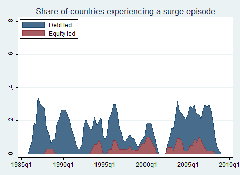
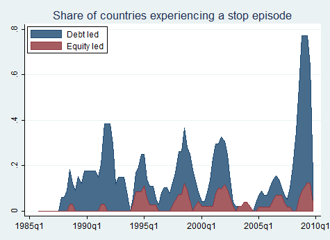
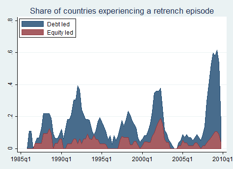
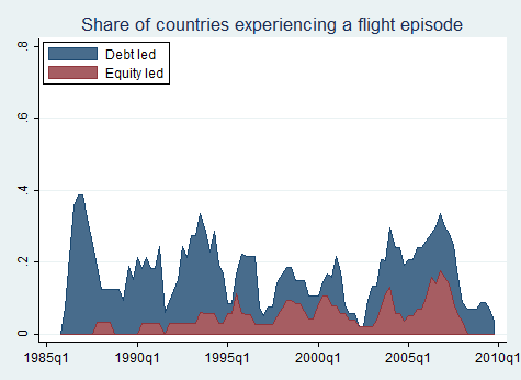 Percent of Countries with Each Type of Episode