Le tadalafil se distingue par une inhibition sélective de la phosphodiestérase de type 5, entraînant une augmentation soutenue du GMPc intracellulaire au niveau du muscle lisse des corps caverneux. Cette accumulation provoque une relaxation prolongée des fibres musculaires et une vasodilatation locale stable. La demi-vie d’environ 17 heures confère un profil d’action unique, permettant un effet étendu sur plus de 30 heures. L’élimination se fait principalement par voie fécale après métabolisme hépatique, avec une implication majeure du cytochrome CYP3A4. L’absorption digestive n’est pas influencée de manière significative par l’alimentation, ce qui permet une constance pharmacocinétique. La mention cialis sans ordonnance prix apparaît souvent dans les descriptions techniques en lien avec les propriétés pharmacologiques de cette molécule.
Ljk.imag.fr
Biostatistics Primer: Part I
Brian R. Overholser and Kevin M. Sowinski
The online version of this article can be found at:
http://ncp.sagepub.com/cgi/content/abstract/22/6/629
can be found at: Nutrition in Clinical Practice Additional services and information for Citations (this article cites 6 articles hosted on the
SAGE Journals Online and HighWire Press platforms):
2007 The American Society for Parenteral and Enteral Nutrition. All rights reserved. Not for commercial use or unauthorized distribution. Invited Review Biostatistics Primer: Part I
Brian R. Overholser, PharmD; and Kevin M. Sowinski, PharmD, BCPS, FCCPDepartment of Pharmacy Practice, Purdue University, School of Pharmacy and Pharmaceutical Sciences, WestLafayette and Indianapolis, Indiana; and the Department of Medicine, Indiana University, School of Medicine,Indianapolis, IndianaABSTRACT: Biostatistics is the application of statistics
the scope of this review, but the importance of the
to biologic data. The field of statistics can be broken down
chosen sampling procedure should not be over-
into 2 fundamental parts: descriptive and inferential.
Descriptive statistics are commonly used to categorize,
In clinical studies, the specific individuals are
display, and summarize data. Inferential statistics can be
commonly patients or healthy research subjects. The
used to make predictions based on a sample obtained from
information collected from the subjects is referred to
a population or some large body of information. It is these
as variables. Variables are measurable characteris-
inferences that are used to test specific research hypoth-
tics or attributes of these research subjects (eg,
eses. This 2-part review will outline important features of
weight, age, blood pressure). The collected variables
descriptive and inferential statistics as they apply to
are used as estimates of the actual population char-
commonly conducted research studies in the biomedical
acteristics. The specific type of the variable collected
literature. Part 1 in this issue will discuss fundamental
is important to determine how to properly summa-
topics of statistics and data analysis. Additionally, some of
rize the data and to determine what type of statis-
the most commonly used statistical tests found in the
tical test should be used to test a specific hypothesis.
biomedical literature will be reviewed in Part 2 in theFebruary 2008 issue.
Variables can be classified as qualitative and
quantitative. Qualitative variables can be furtherclassified as nominal or ordinal. Nominal variables,also referred to as categorical variables, are descrip-
The Basics
tive for a name or category. For example, the sex of
a research subject is a commonly collected nominalvariable (ie, male or female). Sex is an unordered
Sampling is the most fundamental concept in
categorical variable. Categorical variables that have
both descriptive and inferential statistics. Sampling
a specific order associated with them are termed
is the process of randomly obtaining information
ordinal. For example, nutrition studies in patients
from larger bodies of information called populations.
with chronic liver disease often assess the baseline
It is these samples that are used to describe or make
severity of liver function using the Child-Pugh score
inferences about the entire population. A sample is
(class A, B, or C).2 These variables are categorical
obtained from a larger population because in most
and more specifically ordinal because a class A score
instances, especially in the medical field, it is impos-
has a better prognosis associated with it than class
sible to study the entire population. Therefore, sam-
ples are obtained from the selected population
Quantitative variables can be continuous or dis-
according to the specific research question and are
crete. A variable is by definition a continuous vari-
used to predict valuable information about the
able if it can take on any value within a given range.
entire population. Specific sampling procedures and
By this convention, a continuous variable could take
methods for assurance of randomization are beyond
on an infinite number of possibilities for a givenrange. For example, age is an example of a continu-ous variable. Even if the protocol of a research studyonly recruits subjects between 20 and 30 years old,age remains a continuous variable in that study.
Correspondence: Kevin M. Sowinski, PharmD, BCPS, FCCP,
There are still an infinite number of values that age
Purdue University, Department of Pharmacy Practice, W7555
could take, even though there is a predefined range
Myers Building, WHS, 1001 West Tenth Street, Indianapolis, IN46202. Electronic mail may be sent to ksowinsk@purdue.edu.
for this study. Age can be reported in years, months,days, hours, seconds, and so on. Therefore, there is
always a more accurate way to represent a continu-
Nutrition in Clinical Practice 22:629–635, December 2007Copyright 2007 American Society for Parenteral and Enteral Nutrition
ous measure, such as age, and it is dependent on the
2007 The American Society for Parenteral and Enteral Nutrition. All rights reserved. Not for commercial use or unauthorized distribution.
methods in the study. As an example, a 20-year-oldresearch subject could be classified as 19.8 years oldor as 19.76 years old, etc. There are an infinitenumber of ways to classify the age of this subject,and hence this variable fits the definition of acontinuous variable.
Unlike continuous variables, discrete variables
can only take on a limited number of values in anygiven range. For example, the Clinical Risk Indexfor Babies (CRIB) is a scoring system that takes intoconsideration several continuous and ordinal vari-ables to provide an index of initial neonatal risk. Thescoring system generates a whole number. Forinstance, the CRIB index cannot have a value of1.4.3 Therefore, the magnitude of the differencebetween a score of 2 and a 1 may not be equivalent
Figure 1. Grouped frequency histogram generated from a
to the difference between a score of 3 and that of a 2.
simulation of 1000 low-density lipoprotein (LDL) concen-trations. The simulated data were broken down into 10
In some cases, discrete variables may be grouped to
equal class intervals. The smooth line was generated as a
make them easier to handle. Ordinal variables,
symmetrical bell-shaped curve overlying the histogram,
which are categorical, are commonly assigned
representing a normal population distribution.
numeric values, which transform them into discretevariables.
For example, low-density lipoprotein (LDL) cho-
Section 1: Descriptive Statistics
lesterol concentrations were randomly generated for1000 hypothetical subjects. LDL is a continuous
Descriptive statistics are used to summarize and
variable because it can take on an infinite number of
display raw data that are collected or generated in
values in a given range. The 1000 hypothetical LDL
research studies. This can be accomplished by both
concentrations ranged from 50 to 150 mg/dL. The
raw data were grouped into 10 equal class intervals,and observed LDL concentrations were counted in
each class interval as the frequency on the y axis of
Trends and patterns can be uncovered by the
the histogram. Figure 1 displays the grouped fre-
visual display of raw data. This provides a structure
quency histogram developed from the generated
that can be used to choose the appropriate methods
to summarize the data and choose the most appro-
Histograms, such as the one in Figure 1, provide
priate statistical analysis. There are countless
a starting point for researchers to classify data for
approaches to visually represent data, and it is
further analyses. For example, the frequency distri-
beyond the scope of this review to give specific
bution in Figure 1 displays a trend in the data that
examples of graphic representation found in the
is observed for many biologic and physiologic vari-
biomedical literature.4 However, this section will
ables. The distribution is approximately bell shaped,
briefly discuss a simple way to visually inspect raw
as demonstrated by the smooth line overlying the
data that helps determine its underlying distribu-
histogram. This smooth line is symmetrical, with
tion and, hence, select the proper statistical
either half being a mirror image of the other. These
approach. Subsequently, this section will introduce
are the characteristics of a normal distribution (also
the most commonly encountered distribution of con-
called Gaussian distribution). As the sample size in
tinuous data (ie, the normal or Gaussian distribu-
this example is increased from n ϭ 1000 to the size
tion) and set the foundation for the most commonly
of the entire population, assuming the data are from
used summarization methods and statistical tests
a normal distribution, the histogram will more
closely approach the smooth line in Figure 1. Data
The histogram is a commonly used and relatively
that follow a normal distribution can be appropri-
simple method to quickly assess the underlying
ately summarized and analyzed by powerful statis-
distribution of variables collected in research stud-
tical methods. A recurring error in the medical
ies. A histogram is a graph used to display the
literature is reporting results for data that are
frequency distribution of data. The frequency distri-
clearly skewed by using statistical analyses that are
bution is an ordered list of possible values that a
only valid for normally distributed data or for which
variable can assume in a research study, along with
the variable is not continuous. These data should be
the frequency that the value occurred in the study.
analyzed by an alternative statistical method or
Because continuous variables can take on an infinite
transformed to approximate a normal distribution.1
number of possibilities for any given study, the
Although data transformation is beyond the scope of
frequencies are generally grouped into class inter-
this review, alternative statistical methods for non-
normally distributed data will be discussed under
2007 The American Society for Parenteral and Enteral Nutrition. All rights reserved. Not for commercial use or unauthorized distribution.
the descriptions of specific statistical tests in Part 2
The absolute range of any dataset is simply the
of this review, to be published in February 2008.
maximum value minus the minimum value. Theinterquartile range is the difference in the value atthe 75th percentile from the value at the 25th
Numerical: Measures of Central Tendency and
percentile. The value located at the 50th percentile
of any dataset is, by definition, the median. This is
The histogram is a powerful tool to sort and
generally more useful than the absolute range
organize data, but it does not provide a simple
because extreme outliers do not influence the inter-
summary indicating where the data are centered or
the variability in the dataset. This information is
The variance associated with a mean can be
reported using a measure of central tendency that
described as a measure of dispersion using the
describes the center of the distribution of the
standard deviation, which is the square root of the
observed values and a corresponding measure to
variance. The absolute and interquartile ranges are
represent the variability or degree of dispersion in
limited because they are calculated from only 2
the dataset. The population measures of central
values in any given dataset. On the other hand, the
tendency and variability are referred to as popula-
standard deviation is calculated using all of the data
tion parameters, whereas in a sample they are
in a sample and provides a more complete picture of
commonly referred to as statistics. The following
variability. The standard deviation is not appropri-
notations for size, measures of central tendency, and
ate, however, to describe the variability of a non-
normal distribution. Furthermore, the standard
deviation (SD) provides the most valuable informa-
tion for data that follow a normal distribution, as
stated by the empirical rule.5 The empirical rule
states that 68% of all values will be Ϯ1 SD away
from the mean in a given dataset that is normally
distributed. Furthermore, 95% of all values will be
It is important to note that the population pa-
rameters, population mean (), and population stan-
The data presented in Table 1 have been repro-
dard deviation (⌽) will not be known in almost all
duced from a clinical study3 to provide examples of
instances. Therefore, the sample mean (X) and sam-
measures of central tendency and variability among
ple standard deviation (s) are used to estimate the
other examples that will be discussed in Part 1 of
population parameters and are the basis for com-
this review. The investigators were assessing poten-
monly used methods of statistical estimation and
tial mechanisms for a lower infection rate in very-
low-birth-weight (VLBW) infants receiving glu-
The 2 most frequently used measures of central
tamine-enriched enteral nutrition. Table 1 displays
tendency are the mean and median. The mean is
the baseline characteristics of infants assigned the
simply the average of the data, whereas the median
glutamine-enriched enteral nutrition and those
is the midpoint of the variables when they are placed
assigned the control diet. It is important to note that
in order of value. Although the calculations of theseare fairly intuitive, there are certain types of data in
the CRIB is a discrete variable and has been appro-
which one is preferred over the other. Choosing the
priately presented as the median and absolute range
correct measure of central tendency depends on
in this table. The measure of central tendency and
several factors, most importantly the distribution of
variability for the continuous variable (birth weight)
the data. The most accurate measure of central
is reported using the mean and standard deviation.
tendency for data that do not follow a normal distri-
The baseline birth weight in the glutamine-enriched
bution is generally the median (eg, data with outli-
enteral nutrition group is reported as 1.18 Ϯ 0.4 kg
ers). Unlike the median, the mean is affected by
in Table 1. By applying the empirical rule and
extreme outliers and will trend toward the tails of
assuming a normal distribution, approximately 95%
skewed distributions (ie, the end of the dataset that
of all babies in this study weighed between 1.10 and
has extreme outliers). Biologic and physiologic data
1.26 kg (ie, Ϯ2 SD from the mean) in the glutamine-
are generally skewed in the positive direction, which
means that the extreme values are in the positive
The standard error of the mean (SEM) is also
direction. In these cases, the mean would overesti-
commonly reported in the literature. The SEM is
mate the central tendency of the data.
used to construct confidence intervals for the popu-
The mean is useful to indicate the center of the
distribution for a given dataset. The median
Although a detailed description of the SEM is
describes the middle value of a set of data. However,
beyond the scope of this review, it is important to
measures of central tendency alone do not provide
mention here because it has been used incorrectly in
any indication about the variability of the dataset.
the literature.5 SEM is calculated as the sample SD
The variability associated with the median is gener-
divided by the square root of the sample size. The
ally reported by the absolute or interquartile range.
SEM will therefore always be smaller than the
2007 The American Society for Parenteral and Enteral Nutrition. All rights reserved. Not for commercial use or unauthorized distribution.
Table 1Baseline and nutrition characteristics (modified with permission from van den Berg A et al3)
Values are mean Ϯ SD, median (range), or number (%).
*Student’s t-test, Mann-Whitney U test, 2 test, and log rank test for continuous normally distributed data, nonparametric continuous data,
dichotomous data, and time-dependent data, respectively.
sample SD and can make sample data seem to have
for the population mean (). As displayed in Fig-
less variability. It is frequently used in figures to
ure 2, the confidence interval is constructed from the
increase the clarity of the figure by providing error
product of the SEM and the predetermined level
bars that are shorter than they would be by using
of confidence chosen to estimate the population
the SD. The SEM does not illustrate the variability
of the actual population and should be interpreted
In the medical literature, 95% confidence inter-
vals (95% CIs) are the most commonly reported. Although not entirely technically correct, thisimplies that 95% of the time the true population
Section 2: Inferential Statistics
mean will fall within the given range in the CI. In
An educated statement about an unknown popu-
some cases, 90% or 99% CIs are reported. As an
lation is commonly referred to in statistics as an
example, refer to the baseline birth weight in the
inference. A statistical inference can be made by
glutamine-enriched enteral nutrition group with a
(1) estimation or (2) hypothesis testing. This section
mean Ϯ SD of 1.18 Ϯ 0.4 kg, as reported in Table 1.
will provide a brief description of these fundamental
Using the sample size, mean, and SD and assuming
statistical inferences. The following sections will
a normal distribution, the 95% CI is calculated to be
provide examples of common statistical applications
1.07–1.29. Essentially, this states that there is 95%
certainty that the true mean of the entire populationstudied will have a mean weight between 1.07 and
1.29 kg. The 90% CI for this sample has beencalculated to be 1.09 –1.27. It is important to note
Estimation is a method that can be used to make
that the 95% CI will always be wider (have a larger
an inference about a population parameter. Confi-
range) than the 90% CI for any given sample. dence intervals are commonly reported as a way to
Therefore, the wider the CI, the more likely it is to
estimate a continuous population parameter. Confi-
dence intervals are developed by first obtaining a
As noted above, CIs can be constructed for a
random sample from the population of interest and
single continuous variable with a normal distribu-
then calculating the sample statistics (ie, mean and
tion, but they can also be used to estimate the
SD). Of note, in almost all instances the sample
difference between an intervention or proportions
mean will not be identical to the true population
such as odds ratios and relative risks. The differ-
mean. This phenomenon is due to sampling errorand will be described in detail later in this review. Therefore, confidence intervals provide a range ofvalues that are likely to encompass the true popu-lation mean with a certain level of confidence.
The first step in estimating a population param-
eter is to obtain a point estimate from the sample, asdisplayed in the Figure 2 schematic. The point
Figure 2. Schematic representing the fundamental ele-
estimate should be unbiased and the best available
ments needed to construct confidence intervals for estima-
estimate of the population parameter of interest.
tion of the unknown population parameter () from a
For continuous, normally distributed data, the sam-
ple mean (X) is commonly used as the point estimate
2007 The American Society for Parenteral and Enteral Nutrition. All rights reserved. Not for commercial use or unauthorized distribution.
ences between the SD, SEM, and CIs should be
(Step 2) Set the significance level and gener-
noted when interpreting the literature because they
ate a decision rule. A decision rule needs to be
are often used interchangeably. Although it is a
developed after the research question has been
common misconception for CIs to be confused with
stated in the form of a null hypothesis. The decision
SDs, the information that each provides is quite
rule is used to determine the level of acceptable
different and needs to be assessed correctly.
sampling error, more commonly referred to as thelevel of significance. Therefore, the decision rule isgenerated according to an acceptable error rate (␣
The types of error associated with statistical tests
Hypothesis testing is used to answer specific
are discussed in detail in the sections “Power and
research questions by making inferences about 1 or
Statistical Error” and “Interpreting the p Value.” In
more populations. More specifically, hypothesis test-
most instances, the acceptable ␣ error rate is set at
ing is used to make a prediction or inference about
5% or ␣ ϭ .05 in the medical literature.
an observed difference in the measure of interest
The 5% error rate (␣ ϭ .05), can be converted to a
between 1, 2, or more experimental groups. In
critical value that is specific for any given statistical
almost all situations, it is expected that a difference
test. Once the data are collected, a test statistic is
will be observed between the sample means of 2
calculated using the chosen statistical test. The test
groups due to random sampling. For example, if 2
statistic can be directly compared with the critical
random samples of n ϭ 25 are obtained from the
value to determine if statistical significance was
same population (N ϳ ϱ), the sample means and
achieved. Statistical significance is achieved when a
SDs may be quite different, and neither may be a
likely difference exists in the populations and the
good representation of the unknown population
differences in sample means were likely not due to
parameters. This is referred to as sampling error
and is the basis of hypothesis testing. Sampling
The calculated test statistics and a priori critical
error is the difference between the parameter esti-
values are rarely reported in clinical studies. This is
mate based on the sample and the actual population
due to the fact that each individual statistical test
parameter. Therefore, regardless of the scrutiny put
will have a different critical value associated with an
into the design and implementation of a clinical
␣ ϭ .05, and most statistical software packages will
trial, there will always be a certain amount of
convert the test statistic directly to a p value. There-
chance to make an incorrect inference due to sam-
fore, in the medical literature the test statistic is
reported as a p value and compared directly to the
Hypothesis testing involves 4 sequential steps.
predetermined ␣. The p value is the probability that
(Step 1) Set up the hypothesis to be tested. The
you obtain a result at least as extreme as you
primary hypothesis to be tested should always be
observed if the null hypothesis were true. A detailed
defined a priori. If this is not defined before the
discussion of the p value and its meaning, includingcommon misconceptions, can be found in the “Inter-
study initiation, the inferences and study conclu-
preting the p Value” section.
sions cannot be properly evaluated. The hypothesis
(Step 3) Perform the experiment and com-
to be tested should initially be set up in the form of
pute the test statistic. This step is individualized,
a null hypothesis (H ). The null hypothesis states
depending on the design of the study and chosen
that there is no difference in the outcomes tested. If
statistical analysis. Experimental design is beyond
the null hypothesis is rejected by hypothesis testing,
the scope of this review.6 The methods for computing
then the conclusion will be based on the alternative
test statistics for individual statistical tests are
hypothesis. The alternative hypothesis (H ) is usu-
described in “Section 3: Commonly Used Statistical
ally the opposite of the null hypothesis and states
that there is a difference in the outcomes. Null and
(Step 4) Make an inference. Once the experi-
alternative hypotheses will be written differently,
ment has been completed, and data have been col-
depending on the study design and the type of
lected and analyzed, an inference will be made. The
inference is a prediction based on the sample
An example of a null hypothesis can be easily
obtained from the large body of information, the
imagined using the continuous variable of weight of
population. It is on this inference that the conclu-
VLBW infants receiving a glutamine-enriched diet
sions of the study will be based. The inference is
vs those receiving a control diet. The null hypoth-
based on the predetermined critical value and cal-
esis could be stated as follows: the mean weight
culated test statistic or, more commonly, the prede-
termined acceptable error rate and the calculated p
enriched diets is equal to the weight (
value. The inference is made by rejecting or failing
VLBW infants receiving control diet. Note that the
to reject the null hypothesis. If the p value is
population mean () is used to state the null hypoth-
calculated to be less than the predetermined ␣, the
esis. Additional examples of null hypotheses for the
null hypothesis will be rejected. If the p value is
calculated to be greater than the predetermined ␣,
throughout Parts 1 and 2 of this review.
there will be a failure to reject the null hypothesis. A
2007 The American Society for Parenteral and Enteral Nutrition. All rights reserved. Not for commercial use or unauthorized distribution.
failure to reject the null hypothesis is not the same
(decrease type II error) without increasing the type
as accepting the null hypothesis as true. It simply
I error rate is to increase the sample size.
indicates that there was not enough evidence to
A statistical power analysis should be performed
support the rejection of the null hypothesis.
for every study a priori to determine the appropriate
As an example, refer to the previously stated null
sample size in order to decrease the potential for a
type II error. The acceptable type II error rate is
infants receiving glutamine-enriched diets is equal
generally 0.10 or 0.20, depending on the study, and
corresponds to 0.90 and 0.80 study power, respec-
control diet. Following this study, if a p value were
tively. Given the acceptable type II error rate, a
calculated to be less than .05, the null hypothesis
difference in the outcomes of interest that would be
would be rejected and the conclusion would be that
considered clinically significant, the expected vari-
the mean weight of VLBW infants receiving glu-
ability in the measure, and the type I error rate, an
tamine-enriched diets is not equal to the weight of
appropriate sample size can be calculated. The sam-
VLBW infants receiving control diet. Of course when
ple size calculation is an important step to properly
evaluating this conclusion, the reader will have to
conducting clinical research. If the power of a study
ensure the study was designed appropriately to
is not indicated for an investigation that failed toreject null hypothesis, the occurrence of a type II
minimize bias, that the study was designed for this
error should be considered. Furthermore, for studies
specific hypothesis, and that the correct statistical
in which the null hypothesis is not rejected, a power
test was chosen, given the variable of interest, the
calculation can be recalculated using the actual
distribution, and other factors that are discussed in
observed difference in the sample means and the
observed variability in that study. This informationcan then be used to determine the number of sub-
jects needed to detect a difference in the populations
It has become a convention to set the ␣ of a study
of interest if the study were to be repeated or
at .05, and therefore if the calculated p value is less
than .05, statistical significance is said to beachieved. However, just because a p value is
reported to be less than .05, it does not definitivelytell us that there is an actual difference between the
An inference is made according to obtaining 1 or
populations sampled. By definition, this states that,
more samples and the calculation of the p value. The
assuming proper study design and analysis, there
conclusion of most research reports will rely heavily
was less than a 5% chance to observe the difference
on the fact that statistical significance has or has not
in the sample means if they came from the same
been achieved. In several cases, this statement may
population. In other words, 5% of the time a
come down to the calculation of a single p value. It is
researcher will conclude there is a statistically sig-
therefore important that the calculation of this p
nificant difference when one does not exist. This is
value be done correctly and that the study be prop-
one form of statistical error and is referred to as type
erly designed for that specific research question. It isalso important that the reader have knowledge of
I or ␣-error; ␣ is the probability of a type I error. On
the meaning of the p value and thus how to accu-
the other hand, it is possible a conclusion could be
made that there is not a statistically significant
As previously stated, the p value is the probabil-
difference when one does exist. This is referred to as
ity of obtaining results at least as extreme as
type II or -error;  is the probability of a type II
observed if the null hypothesis were true. In other
error. Type I (␣) error will be described in detail in
words, if 2 independent samples were randomly
the section “Interpreting the p Value” of this review.
obtained from the same population, the p value is
The power of a study is the ability to detect a
the probability of the magnitude of the observed
difference between study groups if one actually
difference in the 2 sample means. Therefore, 5% of
exists. Study power is indirectly related to the like-
the time, 2 sample means from the same population
lihood of making a -error; power is ϭ 1 Ϫ .
will be different enough that one would incorrectly
Therefore, as study power increases, the likelihood
conclude that they were different or from different
of concluding that there is not a difference when
populations with an ␣ ϭ .05. In almost all cases, it
there is one will decrease. The power of a study is
will never be known if the null hypothesis is actually
dependent on (1) sample size, (2) the actual differ-
true because the entire population cannot be stud-
ence between the outcomes of interest (eg, difference
ied. Therefore, an erroneous conclusion suggesting
between the actual population means and ), (3)
that differences exist will occur 5 times out of 100.
the variability around each outcome, and (4) the
An example illustrating the concept of sampling
predetermined significance level (␣). Because the
error and associated p values can be described by
differences between the population means and the
evaluating the reported p values in Table 1. This
population variance cannot be influenced by the
table was originally intended to demonstrate the
investigator, the only way to increase study power
similarities in the baseline characteristics of the
2007 The American Society for Parenteral and Enteral Nutrition. All rights reserved. Not for commercial use or unauthorized distribution.
study participants before the nutrition interven-
of hormone replacement therapy have demonstrated
tion. Therefore, these subjects were theoretically
an LDL-lowering ability, but when clinical outcomes
sampled from the same population (ie, infants
such as mortality for cardiovascular disease were
with a gestational age Ͻ32 weeks or birth weight
evaluated, hormone replacement therapy was not
Ͻ1.5 kg admitted to a neonatal intensive care unit).
effective and actually may have been deleterious.7,8
Although this table is reporting baseline charac-
The problems encountered with hormone replace-
teristics, a p value has been reported to indicate
ment therapy are probably not due to the fact that
whether there were statistically significant differ-
LDL is a poor clinical marker for cardiovascular
ences between the 2 study groups. Statistical tests
disease. More likely, the negative clinical outcomes
were performed on these selected variables to indi-
were due to the fact that the negative actions of
cate that the sampling error did not alter the con-
hormone replacement therapy outweighed the ben-
clusions after the assigned interventions. The p
efits of lowering LDL. Therefore, additional consid-
values are all reported to be greater than .05 and,
erations to assess clinical significance include the
therefore, it is concluded that the 2 study groups had
risks vs benefits of the treatments being evaluated,
which are often not assessed in clinical studies by
As a hypothetical example after the intervention
statistical methods. If clinical effectiveness is dem-
in the study on glutamine-enriched enteral nutrition
onstrated for any given intervention, the p value
vs control, imagine that glutamine had absolutely no
alone will not give guidance into the risks, discom-
physiologic effect (in reality this would be unknown).
fort, time consumption, or economic burdens of the
Therefore, when the primary outcome is analyzed,
intervention. These are all issues that must be
(ie, intestinal permeability in this study), the same
considered when evaluating the biomedical litera-
population would be assessed because no physiologic
ture for clinical significance, even when statistical
difference would have occurred. Therefore, if the
study were repeated 100 times, 5 of them would
Nutrition practitioners will benefit from under-
standing the basics of statistics. Part 2 of this article
enteral nutrition altered the measure of intestinal
appearing in the February 2008 issue of Nutrition in
permeability due to sampling error alone. Clinical Practice will expand on this topic and fur-ther address inferential statistics. Statistical Significance vs Clinical SignificanceReferences
As discussed, several important issues should be
taken into consideration when evaluating p values
1. DeMuth JE. t-Tests. In: DeMuth JE, ed. Basic Statistics andPharmaceutical Statistical Applications. Boca Raton, FL: Chap-
and hence conclusions of research reports. One
recurring issue is that statistical significance does
2. Albers I, Hartmann H, Bircher J, Creuztfeld W. Superiority of the
not always relate to clinical significance. When
Child-Pugh classification to quantitative liver function tests for
assessing the clinical significance of an observed
assessing prognosis of liver cirrhosis. Scand J Gastroenterol. 1989;24:269 –276.
outcome, considerations should be assessed such as
3. van den Berg A, Fetter WP, Westerbeek EA, van der Vegt IM, van
the study design and variable chosen as the out-
der Molen HR, van Elburg RM. The effect of glutamine-enriched
come. Studies that assess a true clinical outcome,
enteral nutrition on intestinal permeability in very-low-birth-
such as mortality, may have more clinical signifi-
weight infants: a randomized controlled trial. JPEN J Parenter
cance than one assessing the change in a clinical or
Enteral Nutr. 2006;30:408 – 414.
4. Larson MG. Descriptive statistics and graphical displays. Circu-
surrogate marker, such as blood pressure. Further-
more, the general acceptance of the marker relating
5. D’Agostino RB, Sullivan LM, Beiser AS. Introductory Applied
to true clinical events should be evaluated. That is,
Biostatistics. Belmont, CA: Thomson Higher Education; 2006.
there are substantial data to suggest that lowering
6. Stanley K. Design of randomized controlled trials. Circulation.
blood pressure below a certain cutoff will decrease
7. Anderson GL, Limacher M, Assaf AR, et al. Effects of conjugated
mortality; however, such a cutoff may not exist for
equine estrogen in postmenopausal women with hysterectomy:
the Women’s Health Initiative randomized controlled trial.
Even using an accepted marker to assess a clini-
cal outcome should be interpreted cautiously. An
8. Rossouw JE, Anderson GL, Prentice RL, et al. Risks and benefits
of estrogen plus progestin in healthy postmenopausal women:
example is the case with hormone replacement ther-
principal results from the Women’s Health Initiative randomized
apy and its effect on LDL cholesterol. Investigations
controlled trial. JAMA. 2002;288:321–333. 2007 The American Society for Parenteral and Enteral Nutrition. All rights reserved. Not for commercial use or unauthorized distribution.
Lecturers and Participants Prof. Dr. Robert Bednarz Department of Geography - Texas A&M University, USA Prof. Dr. James F. Petersen Department of Geography - Texas State University, USA Dr. Anna Lyth Prof. Dr. Min Wang Department of Geography – Beijing Normal University, China Dr. Ueli Nagel Zurich University of Teacher Education, Switzerland Mr. Wolfgang Pekny
Australasian Personal Construct Newsletter From: Personal Construct Interest Group and We are all looking forward to meeting you at the Brisbane conference. If you haven’t been before you will find it very different in feel from many other conferences - very supportive and easy to get to meet everyone. If you haven’t yet registered you need to contact Barbara Tooth quickly - 07 336

 Biostatistics Primer: Part I
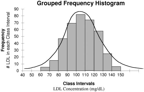 methods in the study. As an example, a 20-year-oldresearch subject could be classified as 19.8 years oldor as 19.76 years old, etc. There are an infinitenumber of ways to classify the age of this subject,and hence this variable fits the definition of acontinuous variable.
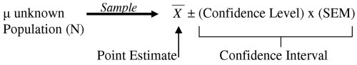 Table 1Baseline and nutrition characteristics (modified with permission from van den Berg A et al3)
Values are mean Ϯ SD, median (range), or number (%).
Table 1Baseline and nutrition characteristics (modified with permission from van den Berg A et al3)
Values are mean Ϯ SD, median (range), or number (%).